Plotting Market Data

pip install matplotlib numpy pands ipykernel
python3 -m ipykernel install --user --name=kraken

from kraken.spot import Market

import matplotlib.pyplot as plt
import numpy as np
import pandas as pd

---

1. Create the unauthenticated market client

market = Market()

2. Get the OHLC data of the XBTUSD pair, create the dataframe, and set the time index

df = pd.DataFrame(
    market.get_ohlc(pair="XBTUSD", interval=60)["XXBTZUSD"],
    columns=["time", "open", "high", "low", "close", "vwap", "volume", "count"],
).astype(float)
# df = df.set_index('time')
df["time"] = pd.to_datetime(df["time"], unit="s")
df = df.sort_values(by="time")
df

	time	open	high	low	close	vwap	volume	count
0	2024-03-02 12:00:00	61917.8	62223.7	61911.4	62142.4	62048.6	15.260659	616.0
1	2024-03-02 13:00:00	62142.4	62142.4	61900.0	61900.0	62006.8	50.357137	727.0
2	2024-03-02 14:00:00	61900.1	61971.8	61663.3	61891.7	61832.5	281.512303	1538.0
3	2024-03-02 15:00:00	61891.8	62032.2	61810.0	61836.8	61941.1	38.815926	886.0
4	2024-03-02 16:00:00	61836.8	62022.3	61714.9	61930.8	61839.0	181.980102	1261.0
...	...	...	...	...	...	...	...	...
715	2024-04-01 07:00:00	69680.1	69788.8	69562.0	69671.7	69676.0	40.187037	767.0
716	2024-04-01 08:00:00	69671.8	69671.8	69244.7	69450.0	69445.2	91.352301	1017.0
717	2024-04-01 09:00:00	69450.1	69613.4	69448.6	69448.7	69510.3	46.275460	731.0
718	2024-04-01 10:00:00	69448.7	69604.4	69353.0	69601.1	69454.0	23.874609	556.0
719	2024-04-01 11:00:00	69601.2	69850.1	69601.1	69666.1	69732.8	20.962756	455.0

720 rows × 8 columns

3. Compute some indicatoes based on the loaded data

# compute ema
df["ema21"] = df["close"].ewm(span=21, adjust=False, min_periods=21).mean()
df["ema50"] = df["close"].ewm(span=50, adjust=False, min_periods=50).mean()
df["ema200"] = df["close"].ewm(span=200, adjust=False, min_periods=200).mean()

def support_and_resistance(df: pd.DataFrame, lookback: int = 200, levels: int = 3) -> dict:
    """Returns up to 3 support and resistance levels by given dataframe"""
    high = df["high"][-lookback:].max()
    low = df["low"][-lookback:].min()
    close = df["close"][-lookback:].iloc[-1]

    pp = (high + low + close) / 3
    s1 = 2 * pp - high
    r1 = 2 * pp - low
    if levels >= 2:
        s2 = pp - (high - low)
        r2 = pp + (high - low)
        if levels >= 3:
            s3 = low - 2 * (high - pp)
            r3 = high + 2 * (pp - low)
            return {"s1": s1, "s2": s2, "s3": s3, "r1": r1, "r2": r2, "r3": r3}
        return {"s1": s1, "s2": s2, "r1": r1, "r2": r2}
    return {"s1": s1, "r2": r1}

# compute support and resistance levels
for i, row in enumerate(df.index):
    try:
        srlevels = support_and_resistance(df.iloc[:i], lookback=50, levels=2)
        df.at[row, "s1"] = srlevels["s1"]
        df.at[row, "r1"] = srlevels["r1"]
        df.at[row, "s2"] = srlevels["s2"]
        df.at[row, "r2"] = srlevels["r2"]
    except:  # noqa: E722
        df.at[row, "s1"] = np.NaN
        df.at[row, "r1"] = np.NaN
        df.at[row, "s2"] = np.NaN
        df.at[row, "r2"] = np.NaN

# isn't that a beauty?:
df

	time	open	high	low	close	vwap	volume	count	ema21	ema50	ema200	s1	r1	s2	r2
0	2024-03-02 12:00:00	61917.8	62223.7	61911.4	62142.4	62048.6	15.260659	616.0	NaN	NaN	NaN	NaN	NaN	NaN	NaN
1	2024-03-02 13:00:00	62142.4	62142.4	61900.0	61900.0	62006.8	50.357137	727.0	NaN	NaN	NaN	61961.300000	62273.600000	61780.200000	62404.800000
2	2024-03-02 14:00:00	61900.1	61971.8	61663.3	61891.7	61832.5	281.512303	1538.0	NaN	NaN	NaN	61792.100000	62115.800000	61684.200000	62331.600000
3	2024-03-02 15:00:00	61891.8	62032.2	61810.0	61836.8	61941.1	38.815926	886.0	NaN	NaN	NaN	61628.766667	62189.166667	61365.833333	62486.633333
4	2024-03-02 16:00:00	61836.8	62022.3	61714.9	61930.8	61839.0	181.980102	1261.0	NaN	NaN	NaN	61592.166667	62152.566667	61347.533333	62468.333333
...	...	...	...	...	...	...	...	...	...	...	...	...	...	...	...
715	2024-04-01 07:00:00	69680.1	69788.8	69562.0	69671.7	69676.0	40.187037	767.0	70380.082934	70315.531093	69369.034227	68659.500000	71012.200000	67639.000000	72344.400000
716	2024-04-01 08:00:00	69671.8	69671.8	69244.7	69450.0	69445.2	91.352301	1017.0	70295.529940	70281.588697	69369.839856	68653.966667	71006.666667	67636.233333	72341.633333
717	2024-04-01 09:00:00	69450.1	69613.4	69448.6	69448.7	69510.3	46.275460	731.0	70218.545400	70248.926395	69370.624534	68506.166667	70858.866667	67562.333333	72267.733333
718	2024-04-01 10:00:00	69448.7	69604.4	69353.0	69601.1	69454.0	23.874609	556.0	70162.414000	70223.521439	69372.917823	68505.300000	70858.000000	67561.900000	72267.300000
719	2024-04-01 11:00:00	69601.2	69850.1	69601.1	69666.1	69732.8	20.962756	455.0	70117.294545	70201.661774	69375.835058	68606.900000	70959.600000	67612.700000	72318.100000

720 rows × 15 columns

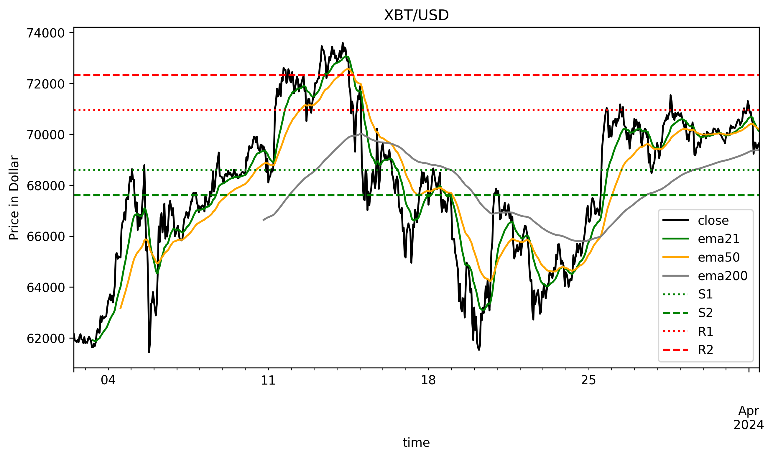
4. Plot the results

fig = plt.figure(figsize=(10, 5), dpi=300)
ax = plt.gca()
df.plot(x="time", y=["close", "ema21", "ema50", "ema200"], ax=ax, color=["black", "green", "orange", "gray"])

xmin, xmax = df["time"].iloc[0], df["time"].iloc[-1]
ax.hlines(y=df["s1"].iloc[-1], xmin=xmin, xmax=xmax, color="green", linestyle=":", label="S1")
ax.hlines(y=df["s2"].iloc[-1], xmin=xmin, xmax=xmax, color="green", linestyle="--", label="S2")
ax.hlines(y=df["r1"].iloc[-1], xmin=xmin, xmax=xmax, color="red", linestyle=":", label="R1")
ax.hlines(y=df["r2"].iloc[-1], xmin=xmin, xmax=xmax, color="red", linestyle="--", label="R2")
ax.set_ylabel("Price in Dollar")
plt.legend()
plt.title("XBT/USD");

… Create and combine custom indicators, implement them, and build your own strategies …